


A signal flow graph is graphical representation of control system. In signal flow graph variables are represented by the nodes of the graph, while relationship between variables are represented by branches connecting nodes.
Signal Flow Graph Terminology:
The different terms used in signal flow graphs are explained below,
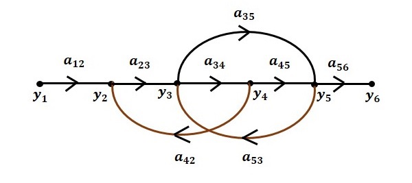
- Node: It is a system variable which is equal to the sum of all incoming signals at the node. Outgoing signals from the node do not affect the value of node variable. For example, consider the signal flow graph shown. Here[tex]{y_1},{y_2},{y_3},{y_4},{y_5},{y_6}[/tex] are nodes. The value of the variable(node)[tex]{y_2}[/tex] given by [tex]{y_2} = {a_{12}}{y_1} + {a_{42}}{y_4}[/tex]
- Branch: A branch is a directed line between nodes.
- Transmittance: Transmittance is gain between nodes or branch gain. Such gains are expressed in terms of transfer function.
- Input node or Source node: It is a node which has only outgoing branches. Here [tex]{y_1}[/tex] is input node.
- Output node or Sink node: It is a node which has only incoming branches. Here [tex]{y_6}[/tex] is output node.
- Chain node or mixed node: It is a node which has both incoming and outgoing branches.
- Path: It is a traversal from one node to another node in the direction of signal(branch arrow), such that no node traverses more than once.
- Forward path: It is a path from the input node to the output node. In the path, [tex]{y_1} \to {y_2} \to {y_3} \to {y_4} \to {y_5} \to {y_6}[/tex] is forward path
- Closed loop: This is a loop which starts from a particular node and ends at the same node. For example, [tex]{y_2} \to {y_3} \to {y_4} \to {y_2}[/tex] form a close path and is called closed loop.
- Self loop: Its also starts from a node and ends at the same node having only one branch.
- Path Gain: It is product of all branch gains in a path. For example,the path gain of the path [tex]{y_1} \to {y_2} \to {y_3} \to {y_5} \to {y_6}[/tex] is[tex]{a_{12}}{a_{23}}{a_{35}}{a_{56}}[/tex].
- Loop gain: It is product of branch gains in a closed loop. For examples, loop gains of loop [tex]{y_2} \to {y_3} \to {y_4} \to {y_2}[/tex] is [tex]{a_{23}}{a_{34}}{a_{42}}[/tex].
- Non touching loop: Loops are said to be non-touching when there are no common nodes between them.
Mason's Gain Formula:
Mason's gain formula is used for the determination of over all transfer function of a system. The number of steps involved in block diagram reduction is high and it is time consuming procedure. Using mason's gain formula is a convenient and easy way of finding the relation between input and output variables.
It is given by,[tex]T = \frac{1}{\Delta }\sum\limits_{i = 1}^K {{P_K}} {\Delta _K}[/tex]
Where, K= number of forward path
[tex]{P_K}[/tex]= path gain of K-th forward path
[tex]\Delta [/tex]= Determinant of the graph
=1-(sum of individual loop gains)+(sum of gain product of all combinations of two non touching
loops)-(sum of gain products of all combinations of three non touching loops)+........
[tex]{\Delta _K}[/tex]= [tex]\Delta [/tex] of part of graph not touching the K-th forward path.
- 1238 views